


반응형
Scatterplot with multiple semantics
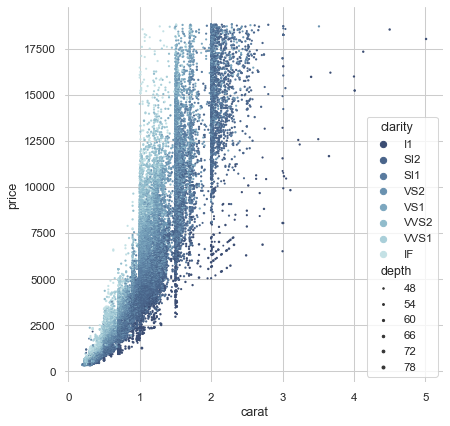
seaborn components used: set_theme(), load_dataset(), despine(), scatterplot()
import seaborn as sns
import matplotlib.pyplot as plt
sns.set_theme(style="whitegrid")

# Load the example diamonds dataset
diamonds = sns.load_dataset("diamonds")

# Draw a scatter plot while assigning point colors and sizes to different
# variables in the dataset
f, ax = plt.subplots(figsize=(6.5, 6.5))
sns.despine(f, left=True, bottom=True)
clarity_ranking = ["I1", "SI2", "SI1", "VS2", "VS1", "VVS2", "VVS1", "IF"]
sns.scatterplot(x="carat", y="price",
                hue="clarity", size="depth",
                palette="ch:r=-.2,d=.3_r",
                hue_order=clarity_ranking,
                sizes=(1, 8), linewidth=0,
                data=diamonds, ax=ax)
Scatterplot with categorical variables
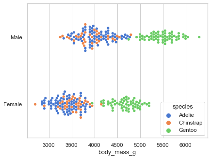
seaborn components used: set_theme(), load_dataset(), swarmplot()
import seaborn as sns
sns.set_theme(style="whitegrid", palette="muted")

# Load the penguins dataset
df = sns.load_dataset("penguins")

# Draw a categorical scatterplot to show each observation
ax = sns.swarmplot(data=df, x="body_mass_g", y="sex", hue="species")
ax.set(ylabel="")
Scatterplot with continuous hues and sizes
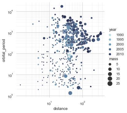
seaborn components used: set_theme(), load_dataset(), cubehelix_palette(), relplot()
import seaborn as sns
sns.set_theme(style="whitegrid")

# Load the example planets dataset
planets = sns.load_dataset("planets")

cmap = sns.cubehelix_palette(rot=-.2, as_cmap=True)
g = sns.relplot(
    data=planets,
    x="distance", y="orbital_period",
    hue="year", size="mass",
    palette=cmap, sizes=(10, 200),
)
g.set(xscale="log", yscale="log")
g.ax.xaxis.grid(True, "minor", linewidth=.25)
g.ax.yaxis.grid(True, "minor", linewidth=.25)
g.despine(left=True, bottom=True)
Scatterplot with varying point sizes and hues
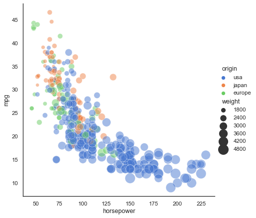
seaborn components used: set_theme(), load_dataset(), relplot()
import seaborn as sns
sns.set_theme(style="white")

# Load the example mpg dataset
mpg = sns.load_dataset("mpg")

# Plot miles per gallon against horsepower with other semantics
sns.relplot(x="horsepower", y="mpg", hue="origin", size="weight",
            sizes=(40, 400), alpha=.5, palette="muted",
            height=6, data=mpg)
Scatterplot Matrix
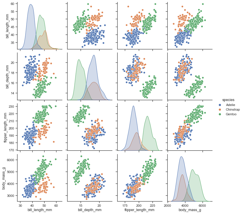
seaborn components used: set_theme(), load_dataset(), pairplot()
import seaborn as sns
sns.set_theme(style="ticks")

df = sns.load_dataset("penguins")
sns.pairplot(df, hue="species")
Plotting model residuals
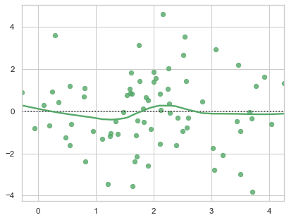
seaborn components used: set_theme(), residplot()
import numpy as np
import seaborn as sns
sns.set_theme(style="whitegrid")

# Make an example dataset with y ~ x
rs = np.random.RandomState(7)
x = rs.normal(2, 1, 75)
y = 2 + 1.5 * x + rs.normal(0, 2, 75)

# Plot the residuals after fitting a linear model
sns.residplot(x=x, y=y, lowess=True, color="g")
Conditional means with observations
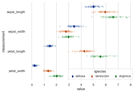
seaborn components used: set_theme(), load_dataset(), despine(), stripplot(), pointplot()
import pandas as pd
import seaborn as sns
import matplotlib.pyplot as plt

sns.set_theme(style="whitegrid")
iris = sns.load_dataset("iris")

# "Melt" the dataset to "long-form" or "tidy" representation
iris = pd.melt(iris, "species", var_name="measurement")

# Initialize the figure
f, ax = plt.subplots()
sns.despine(bottom=True, left=True)

# Show each observation with a scatterplot
sns.stripplot(x="value", y="measurement", hue="species",
              data=iris, dodge=True, alpha=.25, zorder=1)

# Show the conditional means, aligning each pointplot in the
# center of the strips by adjusting the width allotted to each
# category (.8 by default) by the number of hue levels
sns.pointplot(x="value", y="measurement", hue="species",
              data=iris, dodge=.8 - .8 / 3,
              join=False, palette="dark",
              markers="d", scale=.75, ci=None)

# Improve the legend
handles, labels = ax.get_legend_handles_labels()
ax.legend(handles[3:], labels[3:], title="species",
          handletextpad=0, columnspacing=1,
          loc="lower right", ncol=3, frameon=True)
반응형